


We have introduced the terms permittivity of free space, relative and absolute permittivity when we have learned about electric fields; in magnetic circuits the corresponding quantity is the permeability of the material.
If the magnetic field exists in a vacuum, then the ratio of the flux density to the magnetic field strength is a constant, called the permeability of free space, µ0=4πx10-7 henry/metre, and it is used as the reference value from which the permeabilities of all other materials are measured.
Comparing an air-cored solenoid with a fixed value of current flowing it (a certain flux density will be produced by mmf) and a solenoid with an iron core inserted into it, we will find that the flux density will be very much increased. For different core materials there are different results in flux density, and a quantity that describes this is known as relative permeability, same as relative permittivity in electrostatics, µr=B2/B1.
• B1 - the flux density produced in the air
• B2 - the flux density produced in the iron
All non-magnetic materials have the same magnetic properties as a vacuum, µr for air is 1.
The absolute permeability of a material is the ratio of the flux density to magnetic field strength, for a given mmf - µ=B/H [henry/metre], and since µ0 is reference value, it is µ=µ0‧µr, so we have B=µ0‧µr‧H [tesla], which compares directly with D=ε0‧εr‧E [coulomb/m2].
Magnetization (B/H) curve
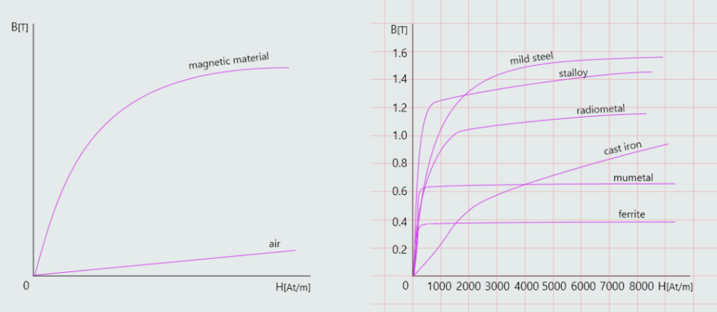
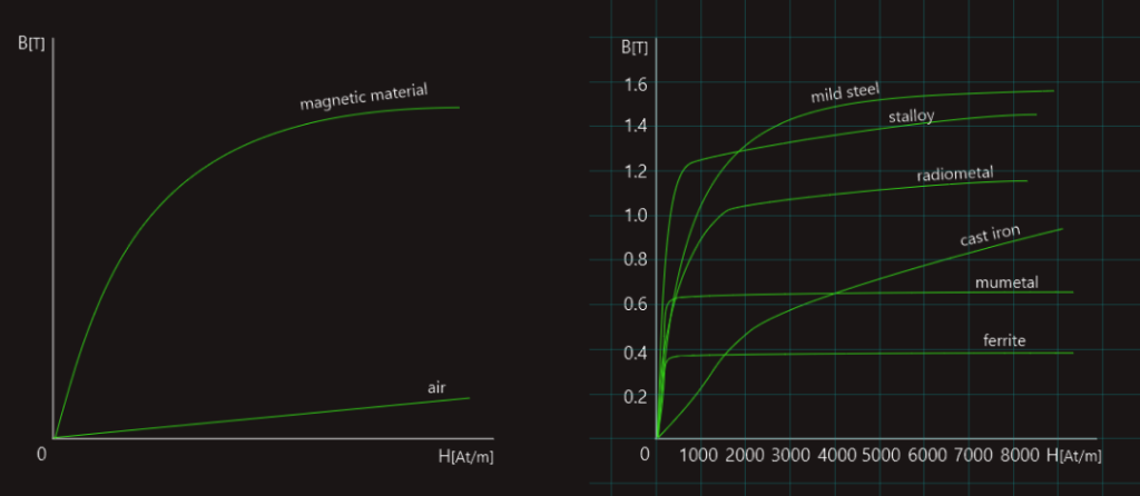
A magnetization curve is a graph of the flux density produced in a magnetic circuit as the magnetic field strength is varied.
Since 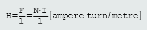 , then for a given magnetic circuit, the field strength may be varied by varying the current through the coil. If the magnetic circuit consists entirely of air, or any other non-magnetic material (µr=1), then the resulting graph will be a straight line passing through the origin; the ratio B/H remains constant. But, the relative permeability of magnetic materials does not remain constant for all values of applied field strength, which results in a curved graph. This non-linearity is due to an effect known as magnetic saturation. We will be dealing here with a much simplified version of this afforded by Ewing’s molecular theory. When the material is unmagnetized, the molecular magnets are orientated in a completely random fashion. This random orientation of the molecular magnets is illustrated in figure below, where the arrows represent the north poles. However, as the coil magnetization current is slowly increased, the molecular magnets start to rotate towards a particular orientation. This results in a certain degree of polarization of the material. As the coil current continues to be increased, the molecular magnets continue to become more aligned. Eventually, the coil current will be sufficient to produce complete alignment. This means that the flux will have reached its maximum possible value. Further increase of the current will produce no further increase of flux. The material is then said to have reached magnetic saturation.
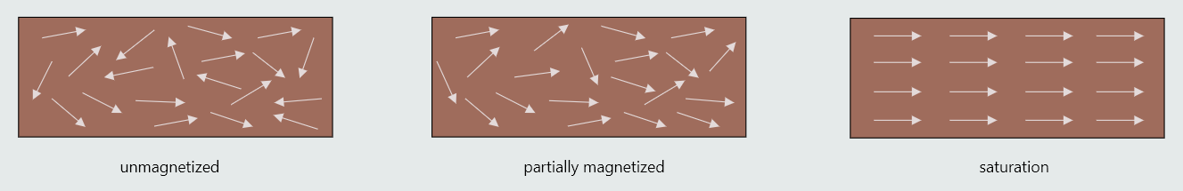
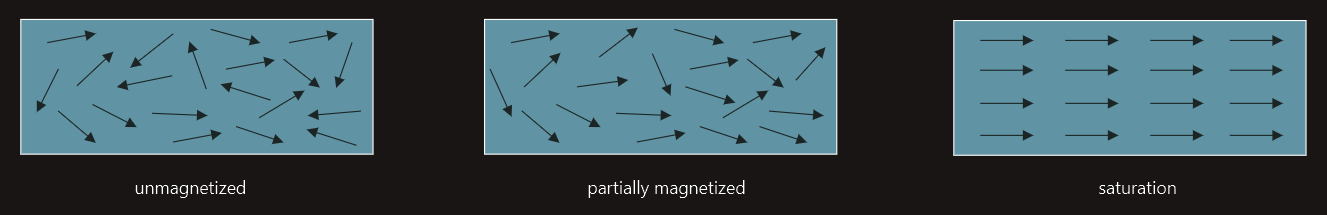
Next two figures show typical magnetization curves for air and a magnetic material, and the magnetization curves for a range of magnetic materials, respectively.
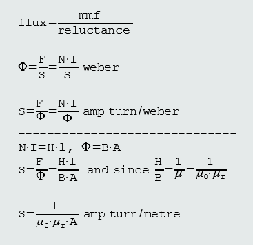
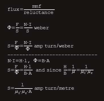
Reluctance (S)
We have already made comparison of magnetic and electric circuit by comparing mmf to emf, flux to current and magnetic field strength to potential gradient. We can make it further by the fact that in magnetic circuit the flux produced by a given mmf is limited by the reluctance of the circuit, same as that the resistance of an electric circuit limits the current that can flow for a given applied emf. So the reluctance of a magnetic circuit is the opposition it offers to the existence of a magnetic flux within it.
While current is a movement of electrons around an electric circuit, a magnetic flux merely exists in a magnetic circuit; it does not involve a flow of particles. However, both current and flux are the direct result of some form of applied force.
We already know that the total resistance in series electrical circuit is the sum of individual resistances, so in magnetic circuit we can also make a comparison and calculate the total reluctance of a series magnetic circuit as S = S1+S2+S3+...
Magnetic flux, also, like most other things in nature tends to take the easiest path available.
For flux this means the lowest reluctance path.
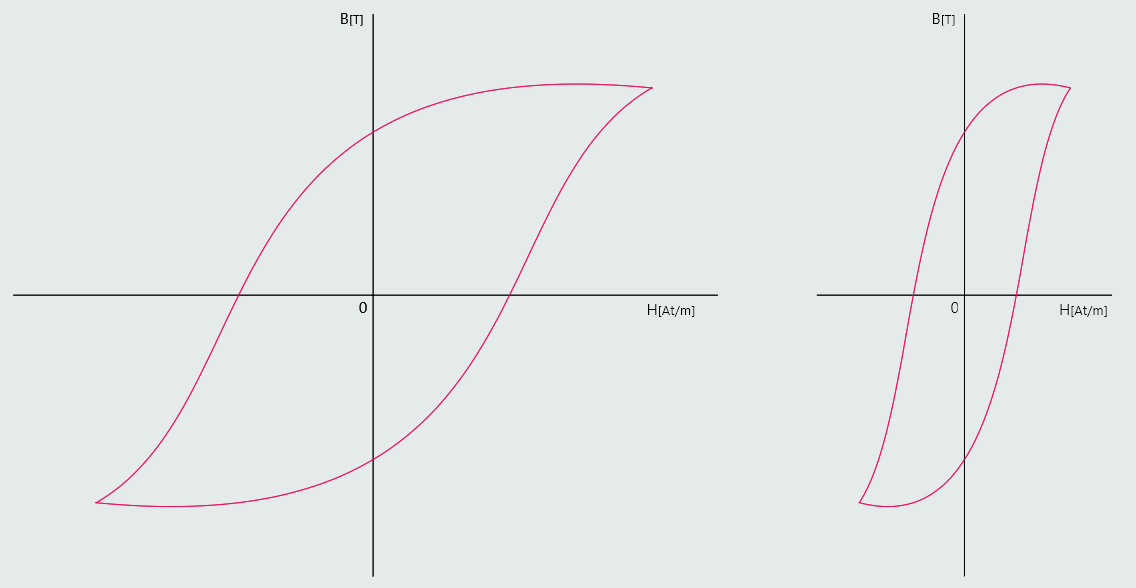
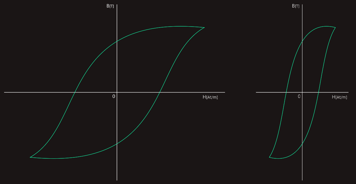
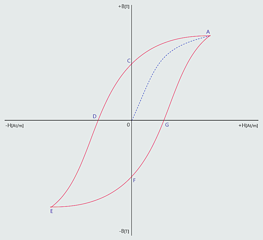
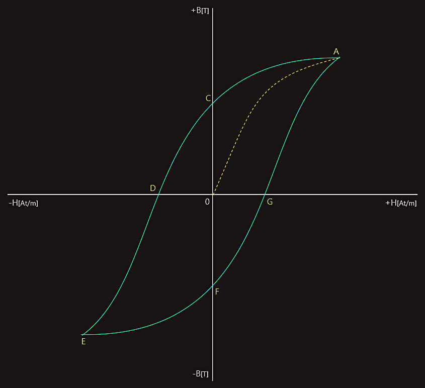
Magnetic Hysteresis
It is found that when the magnetic field strength in a magnetic material is varied, the resulting flux density displays a lagging effect.
Let us now consider magnetic material that initially is completely unmagnetized. If no current flows through the magnetizing coil then both H and B will initially be zero. The value of H is now increased by increasing the coil current in discrete steps. The corresponding flux density is then noted at each step. If these values are plotted on a graph until magnetic saturation is achieved, the dotted curve (the initial magnetization curve) is shown in the figure.
Let the current now be reduced (in steps) to zero, and the corresponding values for B again noted and plotted. This would result in the section of graph from A to C. This shows that when the current is zero once more (so H = 0), the flux density has not reduced to zero. The flux density remaining is called the remanent flux density (OC). This property of a magnetic material, to retain some flux after the magnetizing current is removed, is known as the remanance or retentivity of the material.
Let the current now be reversed, and increased in the opposite direction. This will have the effect of opposing the residual flux. Hence, the latter will be reduced until at some value of - H it reaches zero (point D on the graph). The amount of reverse magnetic field strength required to reduce the residual flux to zero is known as the coercive force. This property of a material is called its coercivity.
If we now continue to increase the current in this reverse direction, the material will once more reach saturation (at point E). In this case it will be of the opposite polarity to that achieved at point A on the graph.
Once again, the current may be reduced to zero, reversed, and then increased in the original direction. This will take the graph from point E back to A, passing through points F and G on the way.
The residual flux density shown as OC has the same value, but opposite polarity, to that shown as OF. Similarly, coercive force OD = OG.
In taking the specimen through the loop ACDEFGA we have taken it through one complete magnetization cycle. The loop is referred to as the hysteresis loop.
Magnetic materials may be subdivided into categories known as ‘hard’ and ‘soft’ magnetic materials. A hard magnetic material is one which possesses a large remanance and coercivity. It is therefore one which retains most of its magnetism, when the magnetizing current is removed. It is also difficult to demagnetize. These are the materials used to form permanent magnets, and they will have a very ‘fat’ loop, as illustrated on the right.
A soft magnetic material, such as soft iron and mild steel, retains very little of the induced magnetism. It will therefore have a relatively ‘thin’ hysteresis loop, as shown on the right, also. The soft magnetic materials are the ones used most often for engineering applications. Examples are the magnetic circuits for rotating electric machines (motors and generators), relays, and the cores for inductors and transformers.
When a magnetic circuit is subjected to continuous cycling through the loop a considerable amount of energy is dissipated. This energy appears as heat in the material. Since this is normally an undesirable effect, the energy dissipated is called the hysteresis loss. Thus, the thinner the loop, the less wasted energy. This is why ‘soft’ magnetic materials are used for the applications that we mentioned above.